The back-and-forth method
This page illustrates the method proposed in A fast approach to optimal transport: The back-and-forth method (Jacobs & Léger, 2020).
We are interested in the optimal transport problem
\[\frac 1 2 W_2(\mu,\nu)^2=\min_{T_{\#}\mu=\nu} \int_{\Omega} \frac 1 2 \lVert T(x)-x\rVert^2 \,\mu(x)dx,\]on the unit square $\Omega=[0,1]^d$ (with $d=2$ or $3$). Here $\mu$ and $\nu$ are two densities on $\Omega$, and $\lVert x-y\rVert^2=(x_1-y_1)^2+(x_2-y_2)^2$.
The approach solves the dual Kantorovich problem
\[\max_{\phi,\psi} \int_{\Omega} \phi(y)\,\nu(y)dy + \int_{\Omega} \psi(x)\,\mu(x)dx,\]over functions $\phi,\psi\colon\Omega\to\mathbb{R}$ satisfying the constraints
\[\phi(y)+\psi(x)\le \frac 1 2 \lVert x-y\rVert^2.\]Code
The code used in the paper is available on GitHub. Documentation available here.
Code was written in C and packaged in both Python and MATLAB.
Python notebook
The simplest way to use the code is to run this Jupyter notebook on Google Colab. Or see it on GitHub.
Videos
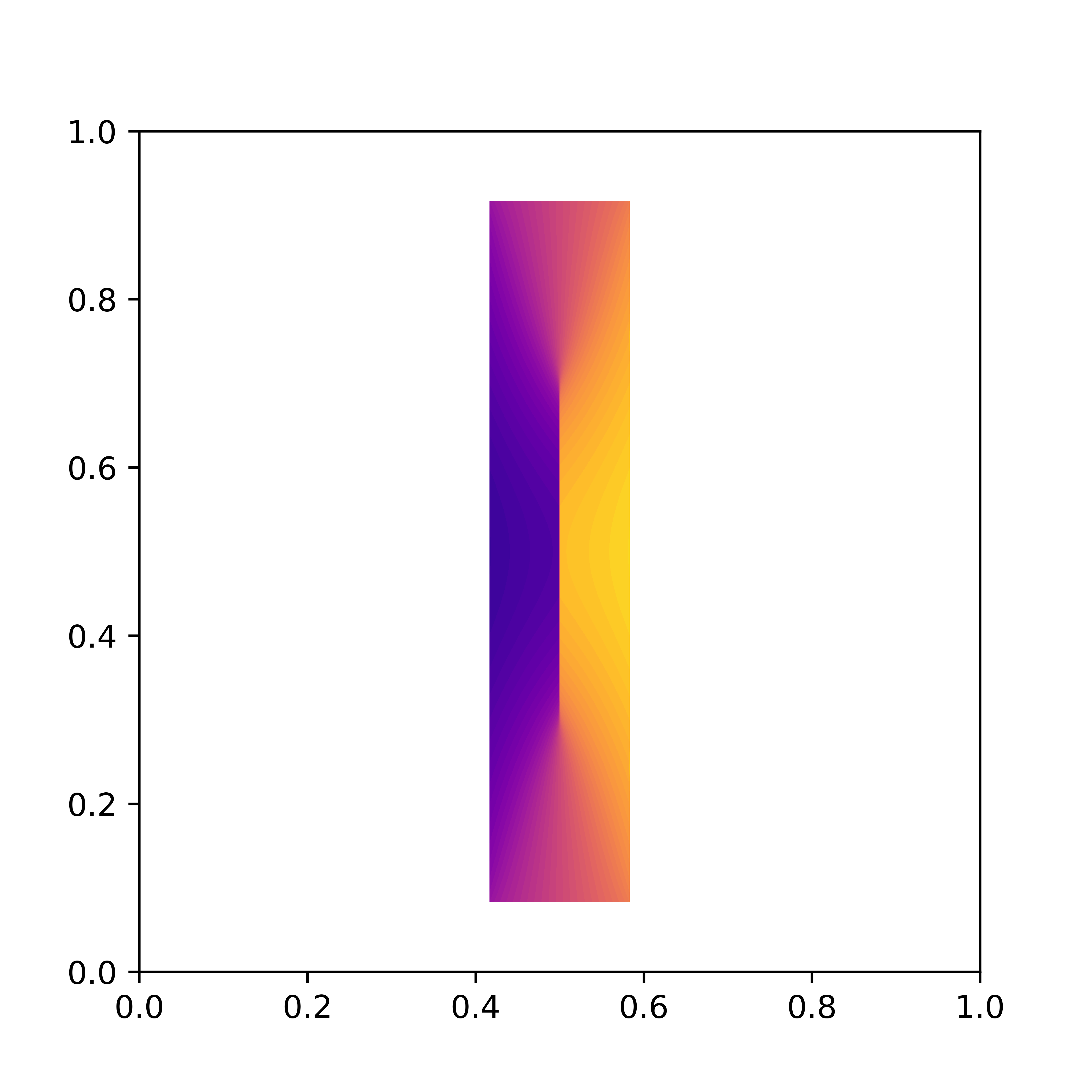
The following videos illustrate displacement interpolation between two probability densities.
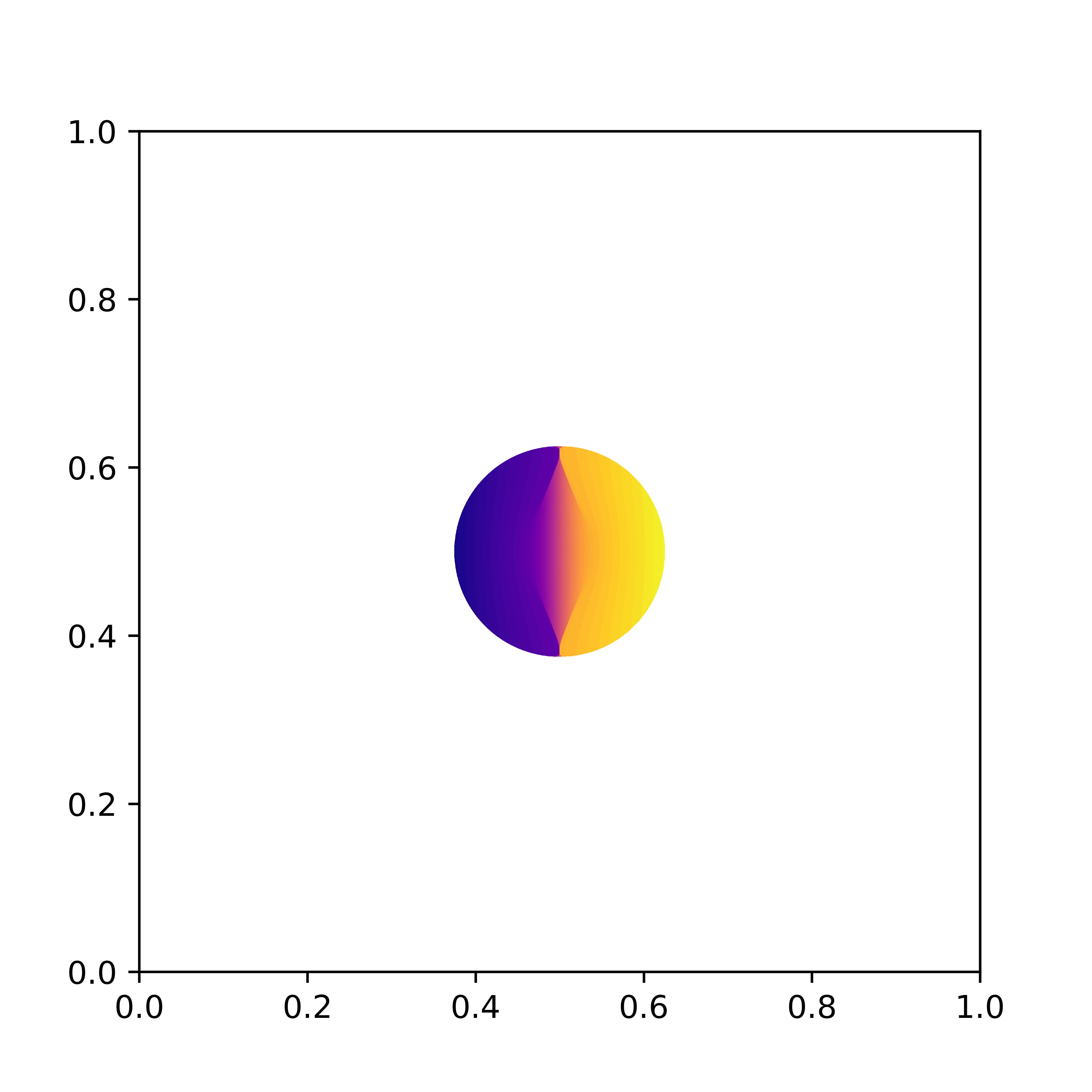
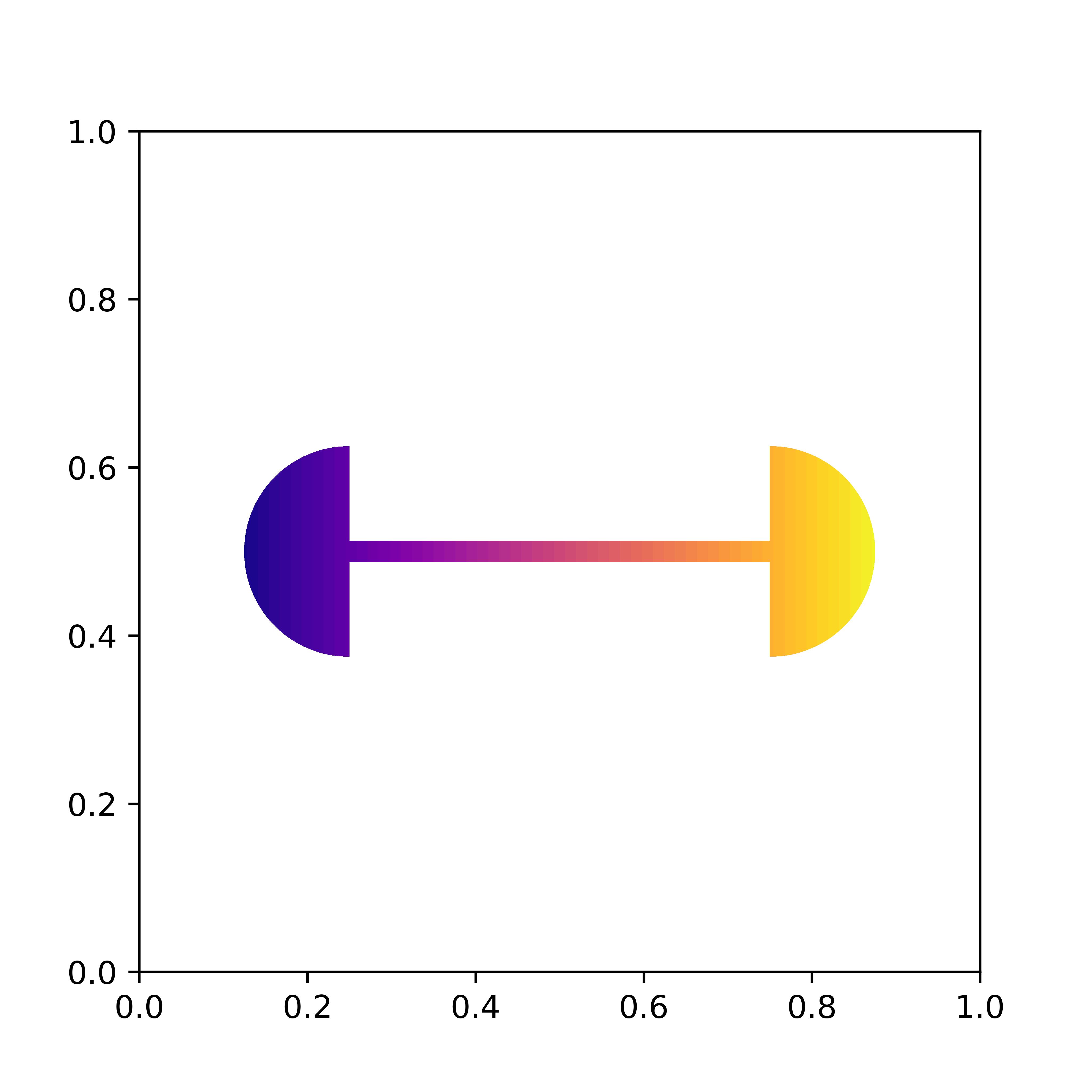
Caffarelli’s counterexample
(Caffarelli, 1992) showed that the optimal transport map can be discontinuous when a measure is supported on a non-convex domain.
Santambrogio–Wang’s counterexample
(Santambrogio & Wang, 2016) showed that the displacement interpolant between two uniform measures supported on convex domains needs not be supported on convex domains. The following shows snapshots at time t=0, t=1/2 and t=1 of their counterexample. Note indeed that the initial and final measures (t=0 and t=1 respectively) are supported on a convex shape (a triangle) while the displacement interpolation at t=1/2 is not.


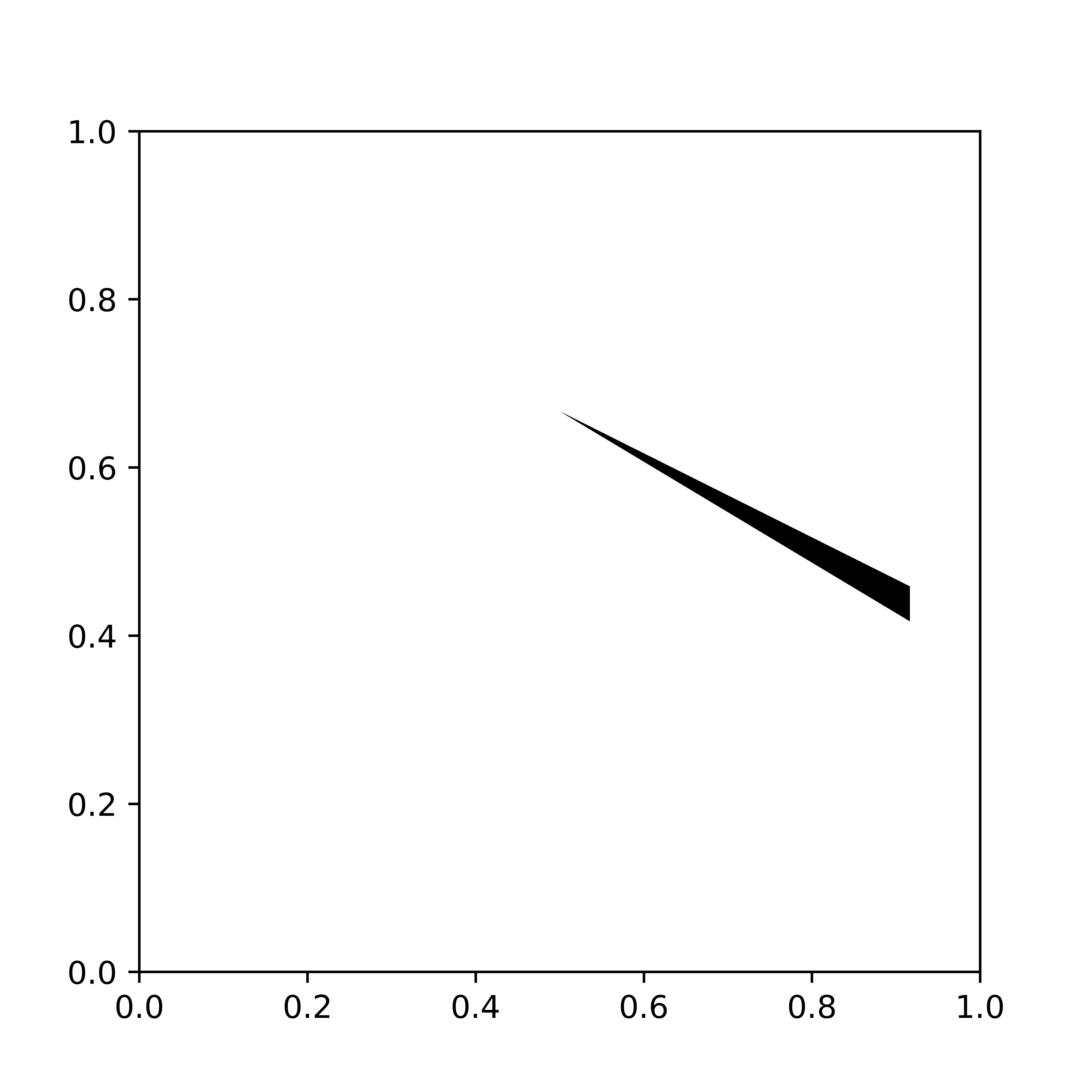
Now we show how mass is transported optimally from the initial density to the final density.

Another example: rectangle to ring
